Math401 Topic 4: The quantum version of probabilistic concepts

In mathematics, on often speaks of non-commutative instead of quantum constructions.

Note, in this section, we will see a lot of mixed used terms used in physics and mathematics. I will use italic to denote the terminology used in physics. It is safe to ignore them if you just care about the mathematics.

Section 1: Generalities about classical versus quantum systems

In classical physics, we assume that a system’s properties have well-defined values regardless of how we choose to measure them.

Basic terminology

Set of states

The preparation of a system builds a convex set of states as our initial condition for the system.

For a collection of $N$ system. Let procedure $N_1=\lambda P_1$ be a preparation procedure for state $P_1$, and $N_2=(1-\lambda) P_2$ be a preparation procedure for state $P_2$. The state of the collection is $N=\lambda N_1+(1-\lambda) N_2$.

Set of effects

The set of effects is the set of all possible outcomes of a measurement. $\Omega=\{\omega_1, \omega_2, \ldots, \omega_n\}$. Where each $\omega_i$ is an associated effect, or some query problems regarding the system. (For example, is outcome $\omega_i$ observed?)

Registration of outcomes

A pair of state and effect determines a probability $E_i(P)=p(\omega_i|P)$. By the law of large numbers, this probability shall converge to $N(\omega_i)/N$ as $N$ increases.

Quantum states, observables (random variables), and effects can be represented mathematically by linear operators on a Hilbert space.

Section 2: Examples of physical experiment in language of mathematics

Sten-Gernach experiment

State preparation: Silver tams are emitted from a thermal source and collimated to form a beam.

Measurement: Silver atoms interact with the field produced by the magnet and impinges on the class plate.

Registration: The impression left on the glass pace by the condensed silver atoms.

Section 3: Finite probability spaces in the language of Hilbert space and operators

Superposition is a linear combination of two or more states.

A quantum coin can be represented mathematically by linear combination of $|0\rangle$ and $|1\rangle$.$\alpha|0\rangle+\beta|1\rangle\in\mathscr{H}\cong\mathbb{C}^2$.

For the rest of the material, we shall take the $\mathscr{H}$ to be vector space over $\mathbb{C}$.

Definitions in classical probability under generalized probability theory

Definition of states (classical probability)

A state in classical probability is a probability distribution on the set of all possible outcomes. We can list as $(p_1,p_2,\cdots,p_n)$.

To each event $A\in \Omega$, we associate the operator on $\mathscr{H}$ of multiplication by the indicator function $P_A\coloneqq M_{\mathbb{I}_A}:f\mapsto \mathbb{I}_A f$ that projects onto the subspace of $\mathscr{H}$ corresponding to the event $A$.

where $a_k\in\{0,1\}$, and $a_k=1$ if and only if $k\in A$. Note that $P_A^*=P_A$ and $P_A^2=P_A$.

Definition of density operator (classical probability)

Let $(p_1,p_2,\cdots,p_n)$ be a probability distribution on $X$, where $p_k\geq 0$ and $\sum_{k=1}^n p_k=1$. The density operator $\rho$ is defined by

The probability of event $A$ relative to the probability distribution $(p_1,p_2,\cdots,p_n)$ becomes the trace of the product of $\rho$ and $P_A$.

Definition of random variables (classical probability)

A random variable is a function $f:X\to\mathbb{R}$. It can also be written in operator form:

The expectation of $f$ relative to the probability distribution $(p_1,p_2,\cdots,p_n)$ is given by

Note, by our definition of the operator $F,P_A,\rho$ (all diagonal operators) commute among themselves, which does not hold in general, in non-commutative (quantum) theory.

Section 4: Why we need generalized probability theory to study quantum systems

Story of light polarization and violation of Bell’s inequality.

Classical picture of light polarization and Bell’s inequality

An interesting story will be presented here.

Polarization of light

The light which comes through a polarizer is polarized in a certain direction. If we fixed the first filter and rotate the second filter, we will observe the intensity of the light will change.

The light intensity decreased with $\alpha$ (the angle between the two filters). The light should vanished when $\alpha=\pi/2$.

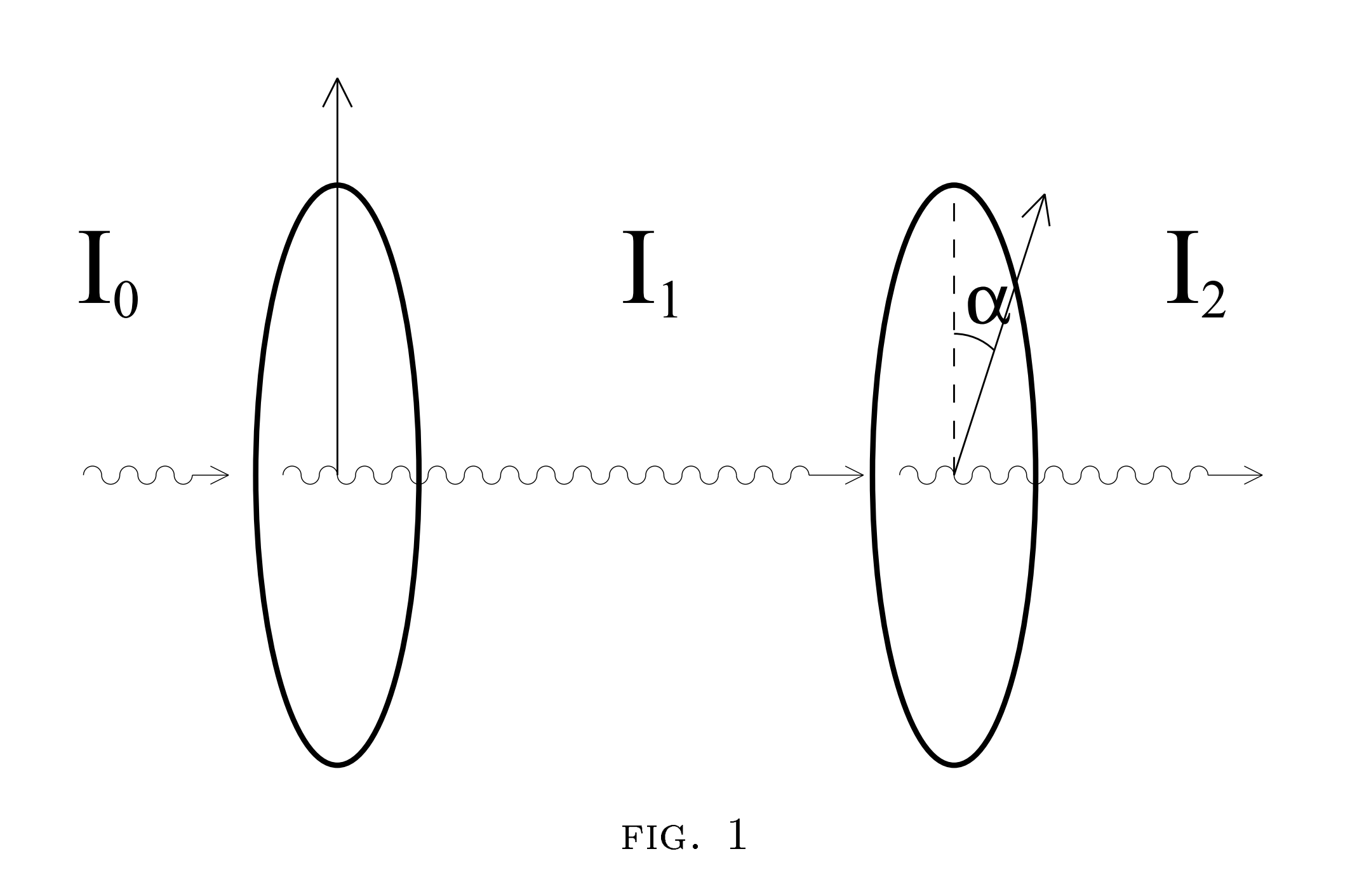
By experimental measurement, the intensity of the light passing the first filter is half the beam intensity (Assume the original beam is completely unpolarized).

Then $I_1=I_0/2$, and

Claim: there exist a smallest package of monochromatic light, which is a photon.

We can model the behavior of each individual photon passing through the filter with direction $\alpha$ with random variable $P_\alpha$. The $P_\alpha(\omega)=1$ if the photon passes through the filter, and $P_\alpha(\omega)=0$ if the photon does not pass through the filter.

Then, the probability of the photon passing through the two filters with direction $\alpha$ and $\beta$ is given by

However, for system of 3 polarizing filters $F_1,F_2,F_3$, having direction $\alpha_1,\alpha_2,\alpha_3$. If we put them on the optical bench in pairs, Then we will have three random variables $P_1,P_2,P_3$.

Bell’s 3 variable inequality

Other revised experiments (eg. Aspect’s experiment, Calcium entangled photon experiment) are also conducted and the inequality is still violated.

The true model of light polarization

The full description of the light polarization is given belows:

State of polarization of a photon: $\psi=\alpha|0\rangle+\beta|1\rangle$, where $|0\rangle$ and $|1\rangle$ are the two orthogonal polarization states in $\mathbb{C}^2$.

Polarization filter (generalized 0,1 valued random variable): orthogonal projection $P_\alpha$ on $\mathbb{C}^2$ corresponding to the direction $\alpha$. (operator satisfies $P_\alpha^*=P_\alpha=P_\alpha^2$.)

The matrix representation of $P_\alpha$ is given by

Probability of a photon passing through the filter $P_\alpha$ is given by $\langle P_\alpha\psi,\psi\rangle$, this is $\cos^2(\alpha)$ if we set $\psi=|0\rangle$.

Since the probability of a photon passing through the three filters is not commutative, it is impossible to discuss $\operatorname{Prob}(P_1=1,P_3=0)$ in the classical setting.

Section 5: The non-commutative (quantum) probability theory

Let $\mathscr{H}$ be a Hilbert space. $\mathscr{H}$ consists of complex-valued functions on a finite set $\Omega=\{1,2,\cdots,n\}$. and that the functions $(e_1,e_2,\cdots,e_n)$ form an orthonormal basis of $\mathscr{H}$. We use Dirac notation $|k\rangle$ to denote the basis vector $e_k$.

In classical settings, multiplication operators is now be the full space of bounded linear operators on $\mathscr{H}$. (Denoted by $\mathscr{B}(\mathscr{H})$)

Let $A,B\in\mathscr{F}$ be the set of all events in the classical probability settings. $X$ denotes the set of all possible outcomes.

A orthogonal projection on a Hilbert space is a projection operator satisfying $P^*=P$ and $P^2=P$. We denote the set of all orthogonal projections on $\mathscr{H}$ by $\mathscr{P}$.

This can be found in linear algebra. Orthogonal projection 

Let $P,Q\in\mathscr{P}$ be the event in non-commutative (quantum) probability space. $R(\cdot)$ is the range of the operator. $P^\perp$ is the orthogonal complement of $P$.

In such setting, some rules of classical probability theory are not valid in quantum probability theory.

In classical probability theory, $A\cap(B\cup C)=(A\cap B)\cup(A\cap C)$.

In quantum probability theory, $P\land(Q\lor R)\neq(P\land Q)\lor(P\land R)$ in general.

Definitions of non-commutative (quantum) probability theory under generalized probability theory

Definition of states (non-commutative (quantum) probability theory)

A state on $(\mathscr{B}(\mathscr{H}),\mathscr{P})$ is a map $\mu:\mathscr{P}\to[0,1]$ such that:

1. $\mu(O)=0$, where $O$ is the zero projection.
2. If $P_1,P_2,\cdots,P_n$ are pairwise disjoint orthogonal projections, then $\mu(P_1\lor P_2\lor\cdots\lor P_n)=\sum_{i=1}^n\mu(P_i)$.

Where projections are disjoint if $P_iP_j=P_jP_i=O$.

Definition of density operator (non-commutative (quantum) probability theory)

A density operator $\rho$ on the finite-dimensional Hilbert space $\mathscr{H}$ is:

1. self-adjoint ($A^*=A$, that is $\langle Ax,y\rangle=\langle x,Ay\rangle$ for all $x,y\in\mathscr{H}$)
2. positive semi-definite (all eigenvalues are non-negative)
3. $\operatorname{Tr}(\rho)=1$.

If $(|\psi_1\rangle,|\psi_2\rangle,\cdots,|\psi_n\rangle)$ is an orthonormal basis of $\mathscr{H}$ consisting of eigenvectors of $\rho$, for the eigenvalue $p_1,p_2,\cdots,p_n$, then $p_j\geq 0$ and $\sum_{j=1}^n p_j=1$.

We can write $\rho$ as

(under basis $|\psi_j\rangle$, it is a diagonal matrix with $p_j$ on the diagonal)

Every basis of $\mathscr{H}$ can be decomposed to these forms.

Theorem: Born’s rule

Let $\rho$ be a density operator on $\mathscr{H}$. then

Defines a probability measure on the space $\mathscr{P}$.

[Proof ignored here]

Theorem: Gleason’s theorem (very important)

Let $\mathscr{H}$ be a Hilbert space over $\mathbb{C}$ or $\mathbb{R}$ of dimension $n\geq 3$. Let $\mu$ be a state on the space $\mathscr{P}$ of projections on $\mathscr{H}$. Then there exists a unique density operator $\rho$ such that

for all $P\in\mathscr{P}$. $\mathscr{P}$ is the space of all orthogonal projections on $\mathscr{H}$.

[Proof ignored here]

Definition of random variable or Observables (non-commutative (quantum) probability theory)

It is the physical measurement of a system that we are interested in. (kinetic energy, position, momentum, etc.)

$\mathscr{B}(\mathbb{R})$ is the set of all Borel sets on $\mathbb{R}$.

An random variable on the Hilbert space $\mathscr{H}$ is a projection valued map $P:\mathscr{B}(\mathbb{R})\to\mathscr{P}$.

With the following properties:

1. $P(\emptyset)=O$ (the zero projection)
2. $P(\mathbb{R})=I$ (the identity projection)
3. For any sequence $A_1,A_2,\cdots,A_n\in \mathscr{B}(\mathbb{R})$. the following holds:
   (a) $P(\bigcup_{i=1}^n A_i)=\bigvee_{i=1}^n P(A_i)$
   (b) $P(\bigcap_{i=1}^n A_i)=\bigwedge_{i=1}^n P(A_i)$
   (c) $P(A^c)=I-P(A)$ (d) If $A_j$ are mutually disjoint (that is $P(A_i)P(A_j)=P(A_j)P(A_i)=O$ for $i\neq j$), then $P(\bigcup_{j=1}^n A_j)=\sum_{j=1}^n P(A_j)$

Definition of probability of a random variable

For a system prepared in state $\rho$, the probability of the random variable by the projection-valued measure $P$ is in the Borel set $A$ is $\operatorname{Tr}(\rho P(A))$.

Expectation of an random variable and projective measurement

Notice that if we set $\lambda$ is observed with probability $p_\lambda=\operatorname{Tr}(\rho P_\lambda)$. $\rho'\coloneqq\sum_{\lambda\in sp(T)}P_\lambda \rho P_\lambda$ is a density operator.

Definition of expectation of operators

Let $T$ be a self-adjoint operator on $\mathscr{H}$. The expectation of $T$ relative to the density operator $\rho$ is given by

if we set $T=\sum_{\lambda\in sp(T)}\lambda P_\lambda$, then $\mathbb{E}_\rho(T)=\sum_{\lambda\in sp(T)}\lambda \operatorname{Tr}(\rho P(\lambda))$.

The uncertainty principle

Let $A,B$ be two self-adjoint operators on $\mathscr{H}$. Then we define the following two self-adjoint operators:

Note that $A\circ B$ satisfies Jordan’s identity.

Definition of variance

Given a state $\rho$, the variance of $A$ is given by

Definition of covariance

Given a state $\rho$, the covariance of $A$ and $B$ is given by the Jordan product of $A$ and $B$.

Robertson-Schrödinger uncertainty relation in finite dimensional Hilbert space

Let $\rho$ be a state on $\mathscr{H}$, $A,B$ be two self-adjoint operators on $\mathscr{H}$. Then

If $\rho$ is a pure state ($\rho=|\psi\rangle\langle\psi|$ for some unit vector $|\psi\rangle\in\mathscr{H}$), and the equality holds, then $A$ and $B$ are collinear (i.e. $A=c B$ for some constant $c\in\mathbb{R}$).

When $A$ and $B$ commute, the classical inequality is recovered (Cauchy-Schwarz inequality).

[Proof ignored here]

The uncertainty relation for unbounded symmetric operators

Definition of symmetric operator

An operator $A$ is symmetric if for all $\phi,\psi\in\mathscr{H}$, we have

An example of symmetric operator is $T(\psi)=i\hbar\frac{d\psi}{dx}$. If we let $\mathscr{H}=\mathscr{D}(T)$, $\hbar$ is the Planck constant.

$\mathscr{D}(T)$ be the space of all square integrable, differentiable, and it’s derivative is also square integrable functions on $\mathbb{R}$.

Definition of joint domain of two operators

Let $(A,\mathscr{D}(A)),(B,\mathscr{D}(B))$ be two symmetric operators on their corresponding domains. The domain of $AB$ is defined as

Since $(AB)\psi=A(B\psi)$, the variance of an operator $A$ relative to a pure state $\rho=|\psi\rangle\langle\psi|$ is given by

If $A$ is symmetric, then $\operatorname{Var}_\rho(A)=\langle A\psi,A\psi\rangle-\langle \psi, A\psi\rangle^2$.

Robertson-Schrödinger uncertainty relation for unbounded symmetric operators

Let $(A,\mathscr{D}(A)),(B,\mathscr{D}(B))$ be two symmetric operators on their corresponding domains. Then

If $\rho$ is a pure state ($\rho=|\psi\rangle\langle\psi|$ for some unit vector $|\psi\rangle\in\mathscr{H}$), and the equality holds, then $A\psi$ and $B\psi$ are collinear (i.e. $A\psi=c B\psi$ for some constant $c\in\mathbb{R}$).

[Proof ignored here]

Summary of analog of classical probability theory and non-commutative (quantum) probability theory

States of two dimensional system and the complex projective space (Bloch sphere)

Let $v=e^{i\theta}u$, then the space of pure states ($\rho=|u\rangle\langle u|$) is the complex projective space $\mathbb{C}P^1$.

$\alpha=x_i+iy_i,\beta=x_2+iy_2$ must satisfy $|\alpha|^2+|\beta|^2=1$, that is $x_1^2+x_2^2+y_1^2+y_2^2=1$.

The set of unit vectors in $\mathbb{C}^2$ is the unit sphere in $\mathbb{R}^3$.

So the space of pure states is the unit circle in $\mathbb{R}^2$.

Mapping between the space of pure states and the complex projective space

Any two dimensional pure state can be written as $e^{i\theta}u$, where $u$ is a unit vector in $\mathbb{R}^2$. There exists a bijective map $P:S^2\to\mathscr{P}_1\subseteq M_2(\mathbb{C})$ such that $P(u)=|u\rangle\langle u|$.